实验三:模型评估与选择(2)
带交叉验证的最优超参数搜索函数
带交叉验证的网格搜索函数
熟悉函数
1 | from sklearn.model_selection import GridSearchCV |
输入参数:
| 参数 | 意义 |
|---|---|
| estimator | 估计器 |
| param_grid | 需要最优化参数的取值(详情见下) |
| scoring | 模型评价标准 |
| refit | 使用在整个数据集上训练的最佳参数重新拟合估计器 |
| cv | 交叉验证的折数(默认 5 折) |
param_grid的形式:- 列表或字典(列表中有多个字典)
- 列表中每项为一个字典,每个字典里键名为需要优化的参数,键值为该参数的取值列表
返回值:
GridSearchCV是一个类,该函数是其构造函数,因此返回的是一个对象,要使用 GridSearch 还需要调用该类中的成员函数fit()
修改参数
实验结果:
| scoring | cv | Best C | Best kernel | best gamma | Best Train | Best Test |
|---|---|---|---|---|---|---|
| accuracy | 5 | 1 | linear | 0.98021978 | 0.96491228 | |
| accuracy | 10 | 100 | linear | 0.98468599 | 0.97368421 | |
| accuracy | 15 | 0.1 | linear | 0.98451613 | 0.97368421 | |
| recall | 5 | 1 | linear | 0.96470588 | 0.96491228 | |
| recall | 10 | 10 | rbf | 0.1 | 0.97647059 | 0.92982456 |
| recall | 15 | 0.1 | linear | 0.96414141 | 0.97368421 | |
| precision | 5 | 0.01 | linear | 1.00000000 | 0.95614035 | |
| precision | 10 | 0.01 | linear | 1.00000000 | 0.95614035 | |
| precision | 15 | 0.001 | linear | 1.00000000 | 0.94736842 | |
| f1 | 5 | 1 | linear | 0.97284941 | 0.96491228 | |
| f1 | 10 | 100 | rbf | 0.001 | 0.97859848 | 0.97368421 |
| f1 | 15 | 0.1 | linear | 0.97802497 | 0.97368421 |
由上图可看出 10 折交叉验证比较通用。适应于大部分情况
带交叉验证的随机搜索函数
熟悉函数
1 | from sklearn.model_selection import RandomizedSearchCV |
输入参数:
| 参数 | 意义 |
|---|---|
| estimator | 估计器 |
| param_distributions | 需要最优化参数的分布(使用 scipy.stats.distributions 里的分布) |
| scoring | 模型评价标准 |
| refit | 使用在整个数据集上训练的最佳参数重新拟合估计器 |
| cv | 交叉验证的折数(默认 5 折) |
返回值:
类似于GridSearchCV
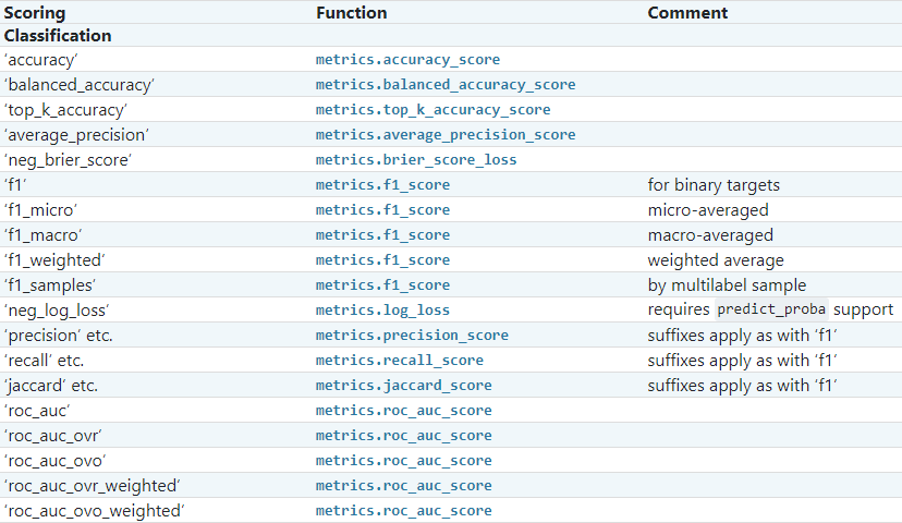
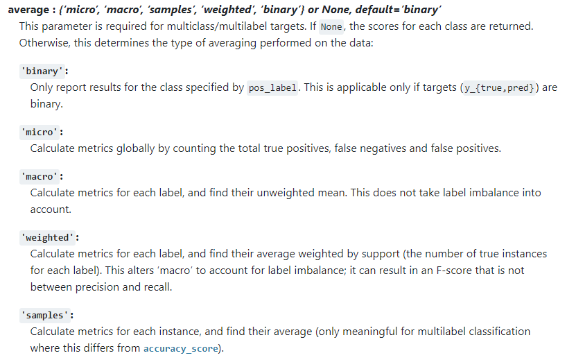
Q: 说明为什么不能使用 ‘recall’, ‘precision’, ‘f1’,而要改为’recall_micro’, ‘precision_micro’, ‘f1_micro’,但是’accuracy’不用加‘_micro’?
A: 以’f1’为例,查阅 SKLearn 文档可知,默认是采用’binary’(二分类),而此时是三分类,默认设置无法使用;而’accuracy’是支持多分类的。
资料来源:
修改参数
以scoring='precision_micro'、cv=8为例,修改C的分布时,可发现其有如下几个最优解:
- 1.668088018810296(0~4 内)
- 5.595344156031953(0~6 内)
- 7.46045887470927(0~8 内)
实验结果:
| scoring | cv | Best C | penalty | Best score(train) |
|---|---|---|---|---|
| accuracy | 5 | 7.011113218 | 11 | 0.98 |
| accuracy | 10 | 7.011113218 | 11 | 0.98 |
| accuracy | 15 | 7.283587054 | 11 | 0.973333333 |
| recall_micro | 5 | 7.011113218 | 11 | 0.98 |
| recall_micro | 10 | 7.011113218 | 11 | 0.98 |
| recall_micro | 15 | 7.283587054 | 11 | 0.973333333 |
| precision_micro | 5 | 7.011113218 | 11 | 0.98 |
| precision_micro | 10 | 7.011113218 | 11 | 0.98 |
| precision_micro | 15 | 7.283587054 | 11 | 0.973333333 |
| f1_micro | 5 | 7.011113218 | 11 | 0.98 |
| f2_micro | 10 | 7.011113218 | 11 | 0.98 |
| f3_micro | 15 | 7.283587054 | 11 | 0.973333333 |
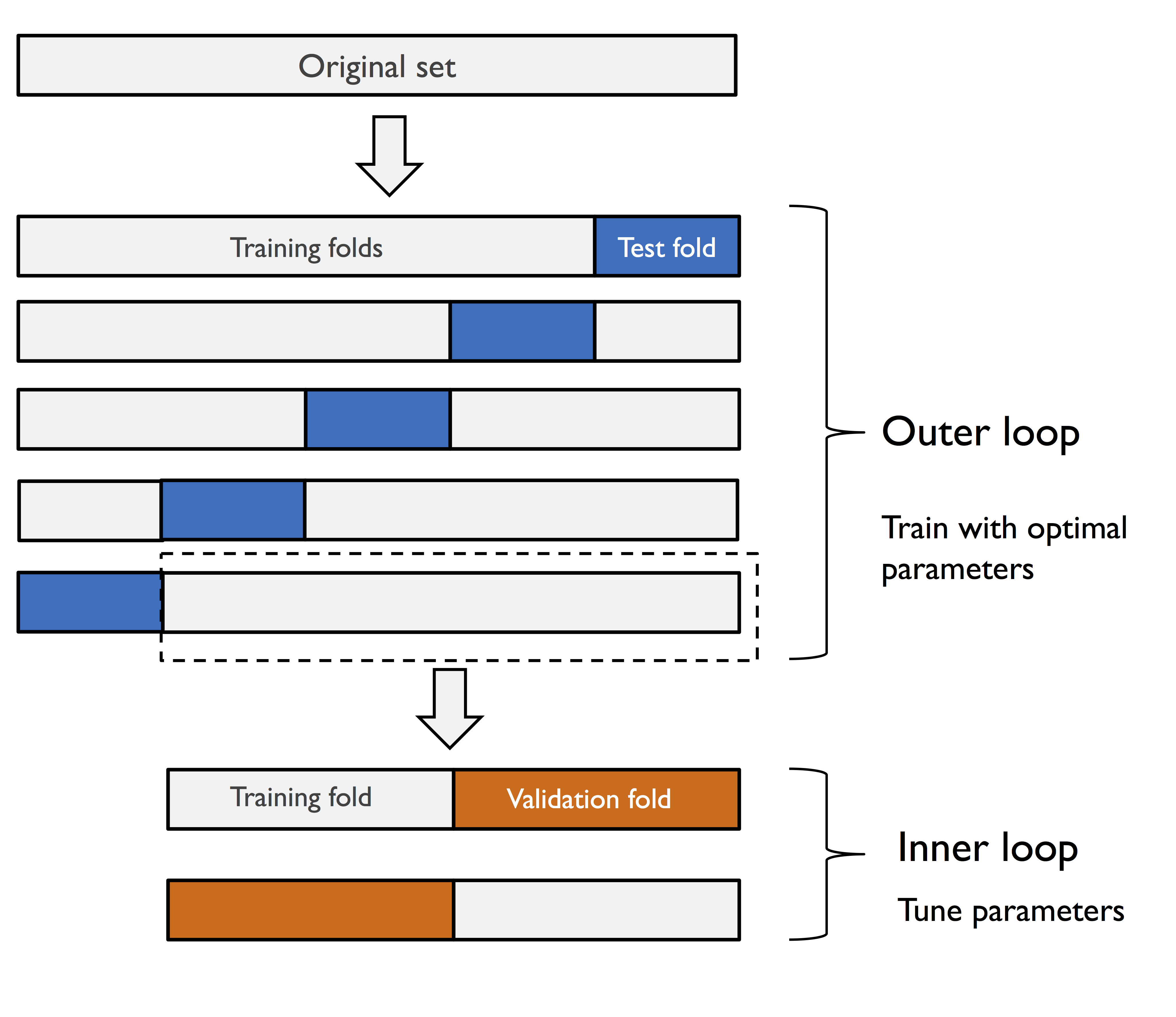
嵌套交叉验证的最优参数搜索方法
熟悉函数
如示例代码:
1 | from sklearn.model_selection import GridSearchCV |
嵌套交叉验证过程:示例代码中先创建GridSearchCV对象gs,再使用cross_val_score()将gs作为估计器,进行交叉验证,从而实现嵌套交叉验证。
在内部交叉验证中优化参数,在外部交叉验证中使用最优参数进行训练
修改参数
运行时使用全部核(R7-5800H),实验结果如下:
| inner cv | outer cv | run time | accuracy | std |
|---|---|---|---|---|
| 3 | 3 | 0.512662 | 0.969 | 0.012 |
| 3 | 5 | 0.835819 | 0.98 | 0.019 |
| 3 | 7 | 1.244654 | 0.982 | 0.025 |
| 3 | 10 | 1.860951 | 0.985 | 0.022 |
| 5 | 3 | 0.874549 | 0.969 | 0.012 |
| 5 | 5 | 1.455379 | 0.971 | 0.023 |
| 5 | 7 | 2.12064 | 0.978 | 0.024 |
| 5 | 10 | 3.27914 | 0.98 | 0.021 |
| 7 | 3 | 1.239511 | 0.969 | 0.012 |
| 7 | 5 | 2.016805 | 0.974 | 0.015 |
| 7 | 7 | 3.094155 | 0.974 | 0.028 |
| 7 | 10 | 4.624048 | 0.978 | 0.02 |
| 10 | 3 | 1.791292 | 0.976 | 0.011 |
| 10 | 5 | 2.894207 | 0.974 | 0.015 |
| 10 | 7 | 4.346896 | 0.98 | 0.024 |
| 10 | 10 | 6.557961 | 0.978 | 0.02 |
从表格中可以看出:准确率和标准差大致随折数增加而增大,但当折数达到一定大小后其变化很小。
其他性能评估指标
混淆矩阵
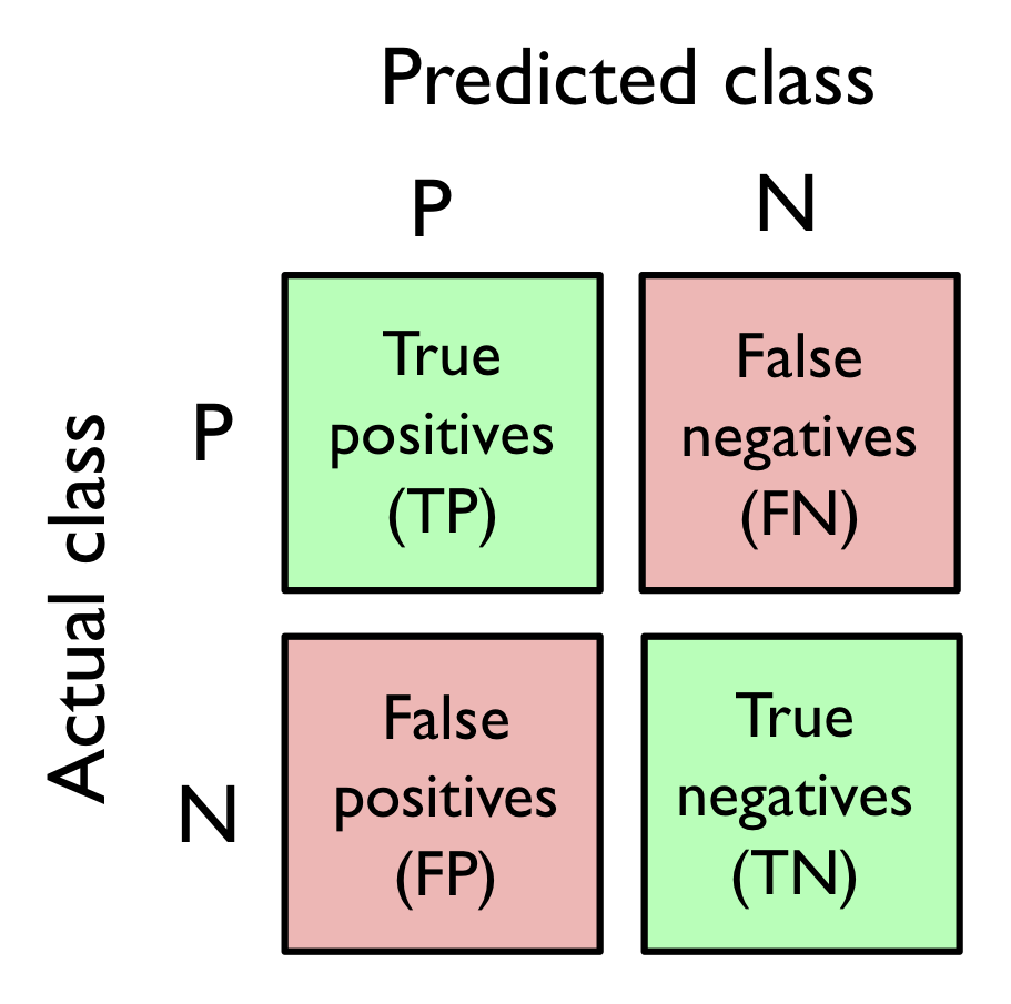
1 | from sklearn.metrics import confusion_matrix |
输入参数:
| 参数 | 意义 |
|---|---|
| y_true | 目标值 |
| y_pred | 估计值 |
返回值:i 行 j 列的矩阵
每格表示真实标签为第 i 类、预测标签为第 j 类的样本数
ROC 曲线
1 | from sklearn.metrics import roc_curve, auc |
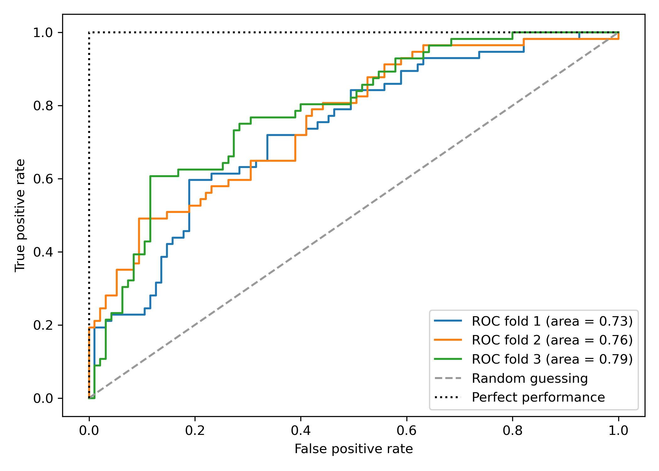
ROC 面积
1 | from sklearn.metrics import roc_curve, auc |
AUC(即 ROC 面积)越大,表示该分类器分类精度越好,AUC 大于 0.5 的分类器才有使用价值。
- AUC=1:完美分类器
- AUC=0.5:与随机分类相同